Features

Data access

Dataset is an abstraction of the local file system. Users can add their local dirs into this system then load data that under these dirs in a convenient way.

XenonPy also uses this system to provide some built-in data. Currently, two sets of element-level property data are available out-of-the-box (elements and elements_completed (imputed version of elements)). These data were collected from mendeleev, pymatgen, CRC Hand Book and Magpie.

elements contains 74 element-level properties of 118 elements. Their missing values were statistically imputed by performing the multiple imputation method [1] and stored as elements_completed. Because of the statistical unreliability of the imputation for a subset of properties and heavier atoms that contains many missing values in elements, the elements_completed data set provides only 58 properties of 94 elements (from H to Pu). The following table shows the currently available elemental information.

Element-level properties

feature	description
period	Period in the periodic table
atomic_number	Number of protons found in the nucleus of an atom
mendeleev_number	Atom number in mendeleev’s periodic table
atomic_radius	Atomic radius
atomic_radius_rahm	Atomic radius by Rahm et al
atomic_volume	Atomic volume
atomic_weight	The mass of an atom
icsd_volume	Atom volume in ICSD database
lattice_constant	Physical dimension of unit cells in a crystal lattice
vdw_radius	Van der Waals radius
vdw_radius_alvarez	Van der Waals radius according to Alvarez
vdw_radius_batsanov	Van der Waals radius according to Batsanov
vdw_radius_bondi	Van der Waals radius according to Bondi
vdw_radius_dreiding	Van der Waals radius from the DREIDING FF
vdw_radius_mm3	Van der Waals radius from the MM3 FF
vdw_radius_rt	Van der Waals radius according to Rowland and Taylor
vdw_radius_truhlar	Van der Waals radius according to Truhlar
vdw_radius_uff	Van der Waals radius from the UFF
covalent_radius_bragg	Covalent radius by Bragg
covalent_radius_cordero	Covalent radius by Cerdero et al
covalent_radius_pyykko	Single bond covalent radius by Pyykko et al
covalent_radius_pyykko_double	Double bond covalent radius by Pyykko et al
covalent_radius_pyykko_triple	Triple bond covalent radius by Pyykko et al
covalent_radius_slater	Covalent radius by Slater
c6	C_6 dispersion coefficient in a.u
c6_gb	C_6 dispersion coefficient in a.u
density	Density at 295K
proton_affinity	Proton affinity
dipole_polarizability	Dipole polarizability
electron_affinity	Electron affinity
electron_negativity	Tendency of an atom to attract a shared pair of electrons
en_allen	Allen’s scale of electronegativity
en_ghosh	Ghosh’s scale of electronegativity
en_pauling	Pauling’s scale of electronegativity
gs_bandgap	DFT bandgap energy of T=0K ground state
gs_energy	DFT energy per atom (raw VASP value) of T=0K ground state
gs_est_bcc_latcnt	Estimated BCC lattice parameter based on the DFT volume
gs_est_fcc_latcnt	Estimated FCC lattice parameter based on the DFT volume
gs_mag_moment	DFT magnetic momenet of T=0K ground state
gs_volume_per	DFT volume per atom of T=0K ground state
hhi_p	Herfindahl−Hirschman Index (HHI) production values
hhi_r	Herfindahl−Hirschman Index (HHI) reserves values
specific_heat	Specific heat at 20oC
gas_basicity	Gas basicity
first_ion_en	First ionisation energy
fusion_enthalpy	Fusion heat
heat_of_formation	Heat of formation
heat_capacity_mass	Mass specific heat capacity
heat_capacity_molar	Molar specific heat capacity
evaporation_heat	Evaporation heat
linear_expansion_coefficient	Coefficient of linear expansion
boiling_point	Boiling temperature
brinell_hardness	Brinell Hardness Number
bulk_modulus	Bulk modulus
melting_point	Melting point
metallic_radius	Single-bond metallic radius
metallic_radius_c12	Metallic radius with 12 nearest neighbors
thermal_conductivity	Thermal conductivity at 25 C
sound_velocity	Speed of sound
vickers_hardness	Value of Vickers hardness test
Polarizability	Ability to form instantaneous dipoles
youngs_modulus	Young’s modulus
poissons_ratio	Poisson’s ratio
molar_volume	Molar volume
num_unfilled	Total unfilled electron
num_valance	Total valance electron
num_d_unfilled	Unfilled electron in d shell
num_d_valence	Valance electron in d shell
num_f_unfilled	Unfilled electron in f shell
num_f_valence	Valance electron in f shell
num_p_unfilled	Unfilled electron in p shell
num_p_valence	Valance electron in p shell
num_s_unfilled	Unfilled electron in s shell
num_s_valence	Valance electron in s shell

For more details on this system, see Data access.

Access https://github.com/yoshida-lab/XenonPy/blob/master/samples/dataset_and_preset.ipynb to get a runnable script.

Descriptor calculation

Compositional descriptors

XenonPy can calculate 290 compositional features for a given chemical composition. This calculation uses the information of the 58 element-level property data recorded in elements_completed. For example, let us consider a binary compound, \(A_{w_A}B_{w_B}\), whose element-level features are denoted by \(f_{A,i}\) and \(f_{B,i} (i = 1, …, 58)\). Then, the 290 compositional descriptors are calculated: for \(i = 1, …, 58\),

• Weighted average (abbr: ave): \(f_{ave, i} = w_{A}^* f_{A,i} + w_{B}^* f_{B,i}\),

• Weighted variance (abbr: var): \(f_{var, i} = w_{A}^* (f_{A,i} - f_{ave, i})^2 + w_{B}^* (f_{B,i} - f_{ave, i})^2\),

• Geometric mean (abbr: gmean): \(f_{gmean, i} = \sqrt[w_A + w_B]{f_{A,i}^{w_A} * f_{V,i}^{w_B}}\),

• Harmonic mean (abbr: hmean): \(f_{hmean, i} = \frac{w_A +w_B}{\frac{1}{f_{A,i}}*w_A + \frac{1}{f_{B,i}}*w_B}\),

• Max-pooling (abbr: max): \(f_{max, i} = max{f_{A,i}, f_{B,i}}\),

• Min-pooling (abbr: min): \(f_{min, i} = min{f_{A,i}, f_{B,i}}\),

• Weighted sum (abbr: sum): \(f_{sum, i} = w_{A} f_{A,i} + w_{B} f_{B,i}\),

where \(w_{A}^*\) and \(w_{B}^*\) denote the normalized composition summing up to one.

By using compositional descriptors, we have succeeded in predicting the composition of quasicrystals [2].

Structural descriptors

Currently, XenonPy implements RDF (radial distribution function) and OFM (orbital field matrix [3]) descriptors of crystalline structures. We also provide a compatible API to use the structural descriptors of matminer. You may check the summary table of featurizers in matminer here.

RDKit descriptors

XenonPy also supports molecular descriptors available in the RDKit python package, including 10 sets of fingerprints, each contains corresponding options.

The tutorial at Descriptor calculation demonstrates how to calculate descriptors using XenonPy.descriptor classes.

Access https://github.com/yoshida-lab/XenonPy/blob/master/samples/calculate_descriptors.ipynb to get a runnable script.

Visualization of descriptor-property relationships

Descriptors on a set of given materials could be displayed on a heatmap plot in order to facilitate the understanding of overall patterns in relation to their properties. The following figure shows an example:

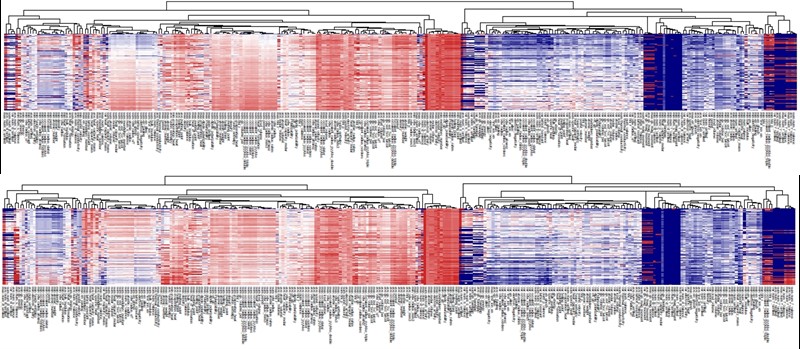
Heatmap of 290 compositional descriptors of 69,640 compounds in Materials Project (upper: volume ų, lower: density g/cm³ ).

In the heatmap of the descriptor matrix, the 69,640 materials are arranged from the top to bottom by the increasing order of formation energies. Plotting the descriptor-property relationships in this way, we could visually recognize which descriptors are relevant or irrelevant to the prediction of formation energies. Relevant descriptors, which are linearly or nonlinearly dependent to formation energies, might exhibit certain patterns from top to bottom in the heatmap. For example, a monotonically decrease or increase pattern would appear in a linearly dependent descriptor. On the other hand, irrelevant descriptors might exhibit no specific patterns.

See the tutorial for visualization of descriptor-property relationships at Visualization.

Access https://github.com/yoshida-lab/XenonPy/blob/master/samples/visualization.ipynb to get a runnable script.

XenonPy.MDL

WARNING: This subsection’s information is out-dated and the details are no long true. Currently XenonPy.MDL is undergoing indefinite maintenance. Please refer to the github README page for the latest update.

XenonPy.MDL is a library of pre-trained models that were obtained by feeding diverse materials data on structure-property relationships into neural networks and some other supervised learning algorithms. The current release (version 0.1.0.beta) contains more than 140,000 models (include private models) on physical, chemical, electronic, thermodynamic, or mechanical properties of small organic molecules (15 properties), polymers/polymer composites (18), and inorganic compounds (12). Pre-trained neural networks are distributed as either the R (MXNet) or Python (PyTorch) model objects. Detailed information about XenonPy.MDL, such as a list of models, properties, source data used for training, and so on, are prepared in this paper [3].

The following lists contain the information of current available pre-trained models and properties.

Information on model sets

id	name	description
1	Stable inorganic compounds in materials project (MP)	Models in this set are trained on ~20,000 stable inorganic compounds selected from the materials project.
2	All inorganic compounds in materials project (MP)	Models in this set are trained on ~70,000 inorganic compounds selected from the materials project.
3	QM9 Dataset from Quantum-Machine website	Quantum-Machine project can be access from http://quantum-machine.org/.
4	PHYSPROP Dataset	PHYSPROP database contains chemical structures, names and physical properties for over 41,000 chemicals.
5	Jean-Claude Bradley Open Melting Point Dataset	Jean-Claude Bradley’s dataset of Open Melting Points.
6	Polymer Genome Dataset (PG)	Polymer Genome is an informatics platform for polymer property prediction and design using machine learning. It can be accessed via https://www.polymergenome.org/.

Information of properties

name	system	querying name
Melting Temperature	Organic Polymer	organic.polymer.melting_temperature
Ionization Energy	Organic Polymer	organic.polymer.ionization_energy
Ionic Dielectric Constant	Organic Polymer	organic.polymer.ionic_dielectric_constant
Hildebrand Solubility Parameter	Organic Polymer	organic.polymer.hildebrand_solubility_parameter
Glass Transition Temperature	Organic Polymer	organic.polymer.glass_transition_temperature
Molar Volume	Organic Polymer	organic.polymer.molar_volume
Electron Affinity	Organic Polymer	organic.polymer.electron_affinity
Dielectric Constant	Organic Polymer	organic.polymer.dielectric_constant
Density	Organic Polymer	organic.polymer.density
Cohesive Energy	Organic Polymer	organic.polymer.cohesive_energy
Bandgap	Organic Polymer	organic.polymer.bandgap
Atomization Energy	Organic Polymer	organic.polymer.atomization_energy
Refractive Index	Organic Polymer	organic.polymer.refractive_index
Molar Heat Capacity	Organic Polymer	organic.polymer.molar_heat_capacity
Electronic Dielectric Constant	Organic Polymer	organic.polymer.electronic_dielectric_constant
U0 Hartree	Organic Nonpolymer	organic.nonpolymer.u0_hartree
R2 Bohr2	Organic Nonpolymer	organic.nonpolymer.r2_bohr2
Mu Debye	Organic Nonpolymer	organic.nonpolymer.mu_debye
Lumo Hartree	Organic Nonpolymer	organic.nonpolymer.lumo_hartree
Homo Hartree	Organic Nonpolymer	organic.nonpolymer.homo_hartree
Gap Hartree	Organic Nonpolymer	organic.nonpolymer.gap_hartree
Alpha Bohr3	Organic Nonpolymer	organic.nonpolymer.alpha_bohr3
U Hartree	Organic Nonpolymer	organic.nonpolymer.u_hartree
Zpve Hartree	Organic Nonpolymer	organic.nonpolymer.zpve_hartree
Bp	Organic Nonpolymer	organic.nonpolymer.bp
Cv Calmol-1K-1	Organic Nonpolymer	organic.nonpolymer.cv_calmol-1k-1
Tm	Organic Nonpolymer	organic.nonpolymer.tm
G Hartree	Organic Nonpolymer	organic.nonpolymer.g_hartree
H Hartree	Organic Nonpolymer	organic.nonpolymer.h_hartree
Density	Inorganic Crystal	inorganic.crystal.density
Volume	Inorganic Crystal	inorganic.crystal.volume
Refractive Index	Inorganic Crystal	inorganic.crystal.refractive_index
Band Gap	Inorganic Crystal	inorganic.crystal.band_gap
Dielectric Const Electron	Inorganic Crystal	inorganic.crystal.dielectric_const_elec
Fermi Energy	Inorganic Crystal	inorganic.crystal.efermi
Total Magnetization	Inorganic Crystal	inorganic.crystal.total_magnetization
Dielectric Const Total	Inorganic Crystal	inorganic.crystal.dielectric_const_total
Final Energy Per Atom	Inorganic Crystal	inorganic.crystal.final_energy_per_atom
Formation Energy Per Atom	Inorganic Crystal	inorganic.crystal.formation_energy_per_atom

XenonPy.MDL provides a rich set of APIs to give users the abilities to interact with the pre-trained model database. Through the APIs, users can search for a specific subset of models by keywords and download them via HTTP. The tutorial at Pre-trained Model Library illustrates how to interact with the database in XenonPy (via the API querying).

Access https://github.com/yoshida-lab/XenonPy/blob/master/samples/pre-trained_model_library.ipynb to get a runnable script.

Transfer learning

Transfer learning has become one of the basic techniques in machine learning that covers a broad range of algorithms for which a model trained for one task is re-purposed to another related task [4] [5]. In general, the need of transfer learning occurs when there is a limited supply of training data for a specific task, yet data supply for related task is sufficient. This situation occurs in many materials science applications as described in [6] [7].

XenonPy offers a simple-to-use toolchain to seamlessly perform transfer learning with the given pre-trained models. Given a target property, by using the transfer learning module of XenonPy, a source model can be treated as a generator of machine learning acquired descriptors, so-called the neural descriptors, as demonstrated in [3].

See tutorial at Transfer Learning to learn how to perform frozen feature transfer learning in XenonPy.

Access https://github.com/yoshida-lab/XenonPy/blob/master/samples/transfer_learning.ipynb to get a runnable script.

Inverse design

Inverse molecular design is an important research subject in materials science that aims to create new chemical structures with desired properties computationally. XenonPy offers a Bayesian molecular design algorithm based on [8] that includes a SMILES generator based on N-gram model, likelihood calculator, and a sequential Monte Carlo algorithm for sampling the posterior distribution of molecules with properties specified by the likelihood function. Details of this algorithm, which is called iQSPR, can be found in [9]. An example of using iQSPR to search for high thermal conductivity polymer can be found in [10].

See tutorial at XenonPy-iQSPR tutorial to learn how to perform inverse molecular design using iQSPR in XenonPy.

Access https://github.com/yoshida-lab/XenonPy/blob/master/samples/iQSPR.ipynb to get a runnable script.

Reference

[1]

4. 2. Rubin, Ed., Multiple Imputation for Nonresponse in Surveys. Hoboken, NJ, USA: John Wiley & Sons, Inc., 1987. doi: 10.1002/9780470316696.

[2]

3. Liu et al., “Machine Learning to Predict Quasicrystals from Chemical Compositions,” Adv. Mater., vol. 33, no. 36, p. 2102507, Sep. 2021, doi: 10.1002/adma.202102507.

[3] (1,2,3)

20. Lam Pham et al., “Machine learning reveals orbital interaction in materials,” Science and Technology of Advanced Materials, vol. 18, no. 1, pp. 756–765, Dec. 2017, doi: 10/gm4znv.

[4]

11. Weiss, T. M. Khoshgoftaar, and D. Wang, “A survey of transfer learning,” J Big Data, vol. 3, no. 1, p. 9, Dec. 2016, doi: 10/gfkr2w.

[5]

3. Tan, F. Sun, T. Kong, W. Zhang, C. Yang, and C. Liu, “A survey on deep transfer learning,” in Artificial neural networks and machine learning – ICANN 2018, Cham, 2018, pp. 270–279.

[6]

8. Yamada et al., “Predicting Materials Properties with Little Data Using Shotgun Transfer Learning,” ACS Cent. Sci., vol. 5, no. 10, pp. 1717–1730, Oct. 2019, doi: 10.1021/acscentsci.9b00804.

[7]

19. Ju et al., “Exploring diamondlike lattice thermal conductivity crystals via feature-based transfer learning,” Phys. Rev. Mater., vol. 5, no. 5, p. 053801, May 2021, doi: 10.1103/physrevmaterials.5.053801.

[8]

8. Ikebata, K. Hongo, T. Isomura, R. Maezono, and R. Yoshida, “Bayesian molecular design with a chemical language model,” J Comput Aided Mol Des, vol. 31, no. 4, pp. 379–391, Apr. 2017, doi: 10/ggpx8b.

[9]

19. Wu, G. Lambard, C. Liu, H. Yamada, and R. Yoshida, “iQSPR in XenonPy: A Bayesian Molecular Design Algorithm,” Mol. Inform., vol. 39, no. 1–2, p. 1900107, Jan. 2020, doi: 10.1002/minf.201900107.

[10]

19. Wu et al., “Machine-learning-assisted discovery of polymers with high thermal conductivity using a molecular design algorithm,” npj Computational Materials, vol. 5, no. 1, pp. 66–66, Dec. 2019, doi: 10.1038/s41524-019-0203-2.