Random NN models

This tutorial shows how to build neural network models. We will learn how to calculate compositional descriptors using xenonpy.descriptor.Compositions calculator and train our model using xenonpy.model.training modules.

In this tutorial, we will use some inorganic sample data from materials project. If you don’t have it, please see https://github.com/yoshida-lab/XenonPy/blob/master/samples/build_sample_data.ipynb.

useful functions

Running the following cell will load some commonly used packages, such as numpy, pandas, and so on. It will also import some in-house functions used in this tutorial. See samples/tools.ipynb to check what will be imported.

[1]:

%run tools.ipynb

Sequential linear model

We will use xenonpy.model.SequentialLinear to build a sequential linear model. The basic layer in SequentialLinear model is xenonpy.model.LinearLayer

[2]:

from xenonpy.model import SequentialLinear, LinearLayer
SequentialLinear?

Init signature:
SequentialLinear(
    in_features: int,
    out_features: int,
    bias: bool = True,
    *,
    h_neurons: Union[Tuple[float, ...], Tuple[int, ...]] = (),
    h_bias: Union[bool, Tuple[bool, ...]] = True,
    h_dropouts: Union[float, Tuple[float, ...]] = 0.1,
    h_normalizers: Union[float, NoneType, Tuple[Union[float, NoneType], ...]] = 0.1,
    h_activation_funcs: Union[Callable, NoneType, Tuple[Union[Callable, NoneType], ...]] = ReLU(),
)
Docstring:
Sequential model with linear layers and configurable other hype-parameters.
e.g. ``dropout``, ``hidden layers``
Init docstring:
Parameters
----------
in_features
    Size of input.
out_features
    Size of output.
bias
    Enable ``bias`` in input layer.
h_neurons
    Number of neurons in hidden layers.
    Can be a tuple of floats. In that case,
    all these numbers will be used to calculate the neuron numbers.
    e.g. (0.5, 0.4, ...) will be expanded as (in_features * 0.5, in_features * 0.4, ...)
h_bias
    ``bias`` in hidden layers.
h_dropouts
    Probabilities of dropout in hidden layers.
h_normalizers
    Momentum of batched normalizers in hidden layers.
h_activation_funcs
    Activation functions in hidden layers.
File:           ~/projects/XenonPy/xenonpy/model/sequential.py
Type:           type
Subclasses:

[3]:

LinearLayer?

Init signature:
LinearLayer(
    in_features: int,
    out_features: int,
    bias: bool = True,
    *,
    dropout: float = 0.0,
    activation_func: Callable = ReLU(),
    normalizer: Union[float, NoneType] = 0.1,
)
Docstring:
Base NN layer. This is a wrap around PyTorch.
See here for details: http://pytorch.org/docs/master/nn.html#
Init docstring:
Parameters
----------
in_features:
    Size of each input sample.
out_features:
    Size of each output sample
dropout: float
    Probability of an element to be zeroed. Default: 0.5
activation_func: func
    Activation function.
normalizer: func
    Normalization layers
File:           ~/projects/XenonPy/xenonpy/model/sequential.py
Type:           type
Subclasses:

Following the official suggestion from PyTorch, SequentialLinear is a python class that inherit the torch.nn.Module class. Users can specify the hyperparameters to get a fully customized model object. For example:

[4]:

model = SequentialLinear(290, 1, h_neurons=(0.8, 0.7, 0.6))
model

[4]:

SequentialLinear(
  (layer_0): LinearLayer(
    (linear): Linear(in_features=290, out_features=232, bias=True)
    (dropout): Dropout(p=0.1)
    (normalizer): BatchNorm1d(232, eps=0.1, momentum=0.1, affine=True, track_running_stats=True)
    (activation): ReLU()
  )
  (layer_1): LinearLayer(
    (linear): Linear(in_features=232, out_features=203, bias=True)
    (dropout): Dropout(p=0.1)
    (normalizer): BatchNorm1d(203, eps=0.1, momentum=0.1, affine=True, track_running_stats=True)
    (activation): ReLU()
  )
  (layer_2): LinearLayer(
    (linear): Linear(in_features=203, out_features=174, bias=True)
    (dropout): Dropout(p=0.1)
    (normalizer): BatchNorm1d(174, eps=0.1, momentum=0.1, affine=True, track_running_stats=True)
    (activation): ReLU()
  )
  (output): Linear(in_features=174, out_features=1, bias=True)
)

fully randomized model generation

Process of random model generation:

using a random parameter generator to generate a set of parameter.
using the generated parameter set to setup a model object.
loop step 1 and 2 as many times as needed.

We provided a general parameter generator xenonpy.utils.ParameterGenerator to do all the 3 steps for any callable object.

[5]:

from xenonpy.utils import ParameterGenerator
ParameterGenerator?

Init signature:
ParameterGenerator(
    seed: Union[int, NoneType] = None,
    **kwargs: Union[Any, Sequence, Callable, Dict],
)
Docstring:      Generator for parameter set generating.
Init docstring:
Parameters
----------
seed
    Numpy random seed.
kwargs
    Parameter candidate.
File:           ~/projects/XenonPy/xenonpy/utils/parameter_gen.py
Type:           type
Subclasses:

Calling an instance of ParameterGenerator will return a generator. This generator can randomly select parameters from parameter candidates and yield them as a dict. This is what we want in step 1.

[6]:

from math import ceil
from random import uniform

generator = ParameterGenerator(
    in_features=290,
    out_features=1,
    h_neurons=dict(
        data=[ceil(uniform(0.1, 1.2) * 290) for _ in range(100)],
        repeat=(2, 3)
    )
)

Because generator is a generator, for ... in ... statement can be applied. For example, we can use for parameters in generator(num_of_models) to loop all these generated parameter sets.

[7]:

for parameters in generator(num=10):
    print(parameters)

{'in_features': 290, 'out_features': 1, 'h_neurons': (70, 109)}
{'in_features': 290, 'out_features': 1, 'h_neurons': (135, 45)}
{'in_features': 290, 'out_features': 1, 'h_neurons': (216, 261, 79)}
{'in_features': 290, 'out_features': 1, 'h_neurons': (111, 88, 49)}
{'in_features': 290, 'out_features': 1, 'h_neurons': (216, 79, 47)}
{'in_features': 290, 'out_features': 1, 'h_neurons': (161, 45)}
{'in_features': 290, 'out_features': 1, 'h_neurons': (193, 161, 78)}
{'in_features': 290, 'out_features': 1, 'h_neurons': (90, 36, 234)}
{'in_features': 290, 'out_features': 1, 'h_neurons': (230, 83, 295)}
{'in_features': 290, 'out_features': 1, 'h_neurons': (171, 247)}

For step 2, we can give a model class to the factory parameter as a factory function. If factory parameter is given, generator will feed generated parameters to the factory function automatically and yield the result as a second return in each loop. For example:

[8]:

for parameters, model in generator(2, factory=SequentialLinear):
    print('parameters: ', parameters)
    print(model, '\n')

parameters:  {'in_features': 290, 'out_features': 1, 'h_neurons': (182, 335, 204)}
SequentialLinear(
  (layer_0): LinearLayer(
    (linear): Linear(in_features=290, out_features=182, bias=True)
    (dropout): Dropout(p=0.1)
    (normalizer): BatchNorm1d(182, eps=0.1, momentum=0.1, affine=True, track_running_stats=True)
    (activation): ReLU()
  )
  (layer_1): LinearLayer(
    (linear): Linear(in_features=182, out_features=335, bias=True)
    (dropout): Dropout(p=0.1)
    (normalizer): BatchNorm1d(335, eps=0.1, momentum=0.1, affine=True, track_running_stats=True)
    (activation): ReLU()
  )
  (layer_2): LinearLayer(
    (linear): Linear(in_features=335, out_features=204, bias=True)
    (dropout): Dropout(p=0.1)
    (normalizer): BatchNorm1d(204, eps=0.1, momentum=0.1, affine=True, track_running_stats=True)
    (activation): ReLU()
  )
  (output): Linear(in_features=204, out_features=1, bias=True)
)

parameters:  {'in_features': 290, 'out_features': 1, 'h_neurons': (108, 255)}
SequentialLinear(
  (layer_0): LinearLayer(
    (linear): Linear(in_features=290, out_features=108, bias=True)
    (dropout): Dropout(p=0.1)
    (normalizer): BatchNorm1d(108, eps=0.1, momentum=0.1, affine=True, track_running_stats=True)
    (activation): ReLU()
  )
  (layer_1): LinearLayer(
    (linear): Linear(in_features=108, out_features=255, bias=True)
    (dropout): Dropout(p=0.1)
    (normalizer): BatchNorm1d(255, eps=0.1, momentum=0.1, affine=True, track_running_stats=True)
    (activation): ReLU()
  )
  (output): Linear(in_features=255, out_features=1, bias=True)
)

We also enable users to generate parameters in a functional way by given a function as candidate parameters. In this case, the function accept an int number as vector length and a vector of generated parameters. For example, generate a n length vector with float numbers sorted in ascending.

[9]:

generator = ParameterGenerator(
    in_features=290,
    out_features=1,
    h_neurons=dict(
        data=lambda n: sorted(np.random.uniform(0.2, 0.8, size=n), reverse=True),
        repeat=(2, 3)
    )
)

[10]:

for parameters, model in generator(2, factory=SequentialLinear):
    print('parameters: ', parameters)
    print(model, '\n')

parameters:  {'in_features': 290, 'out_features': 1, 'h_neurons': (0.7954011465554711, 0.6993610045591458)}
SequentialLinear(
  (layer_0): LinearLayer(
    (linear): Linear(in_features=290, out_features=231, bias=True)
    (dropout): Dropout(p=0.1)
    (normalizer): BatchNorm1d(231, eps=0.1, momentum=0.1, affine=True, track_running_stats=True)
    (activation): ReLU()
  )
  (layer_1): LinearLayer(
    (linear): Linear(in_features=231, out_features=203, bias=True)
    (dropout): Dropout(p=0.1)
    (normalizer): BatchNorm1d(203, eps=0.1, momentum=0.1, affine=True, track_running_stats=True)
    (activation): ReLU()
  )
  (output): Linear(in_features=203, out_features=1, bias=True)
)

parameters:  {'in_features': 290, 'out_features': 1, 'h_neurons': (0.798810246990777, 0.38584535382368323, 0.29569841893337045)}
SequentialLinear(
  (layer_0): LinearLayer(
    (linear): Linear(in_features=290, out_features=232, bias=True)
    (dropout): Dropout(p=0.1)
    (normalizer): BatchNorm1d(232, eps=0.1, momentum=0.1, affine=True, track_running_stats=True)
    (activation): ReLU()
  )
  (layer_1): LinearLayer(
    (linear): Linear(in_features=232, out_features=112, bias=True)
    (dropout): Dropout(p=0.1)
    (normalizer): BatchNorm1d(112, eps=0.1, momentum=0.1, affine=True, track_running_stats=True)
    (activation): ReLU()
  )
  (layer_2): LinearLayer(
    (linear): Linear(in_features=112, out_features=86, bias=True)
    (dropout): Dropout(p=0.1)
    (normalizer): BatchNorm1d(86, eps=0.1, momentum=0.1, affine=True, track_running_stats=True)
    (activation): ReLU()
  )
  (output): Linear(in_features=86, out_features=1, bias=True)
)

Model training

We provide a general and extendable model training system for neural network models. By customizing the extensions, users can fully control their model training process, and save the training results following the XenonPy.MDL format automatically.

All these modules and extensions are under the xenonpy.model.training.

[11]:

import torch
import matplotlib.pyplot as plt
from pymatgen import Structure

from xenonpy.model.training import Trainer, SGD, MSELoss, Adam, ReduceLROnPlateau, ExponentialLR, ClipValue

from xenonpy.datatools import preset, Splitter
from xenonpy.descriptor import Compositions

prepare training/testing data

If you followed the tutorial in https://github.com/yoshida-lab/XenonPy/blob/master/samples/build_sample_data.ipynb, the sample data should be save at ~/.xenonpy/userdata with name mp_samples.pd.xz. You can use pd.read_pickle to load this file but we suggest that you use our xenonpy.datatools.preset module.

We chose volume as the example to demonstrate how to use our training system. We only use the data which volume are smaller than 2,500 to avoid the disparate data. we select data in pandas.DataFrame and calculate the descriptors using xenonpy.descriptor.Compositions calculator. It is noticed that the input for a neuron network model in pytorch must has shape (N x M x …), which mean if the input is a 1-D vector, it should be reshaped to 2-D, e.g. (N) -> (N x 1).

[12]:

# if you have not have the samples data
# preset.build('mp_samples', api_key=<your materials project api key>)

from xenonpy.datatools import preset

data = preset.mp_samples
data.head(3)

[12]:

	band_gap	composition	density	e_above_hull	efermi	elements	final_energy_per_atom	formation_energy_per_atom	pretty_formula	structure	volume
mp-1008807	0.0000	{'Rb': 1.0, 'Cu': 1.0, 'O': 1.0}	4.784634	0.996372	1.100617	[Rb, Cu, O]	-3.302762	-0.186408	RbCuO	[[-3.05935361 -3.05935361 -3.05935361] Rb, [0....	57.268924
mp-1009640	0.0000	{'Pr': 1.0, 'N': 1.0}	8.145777	0.759393	5.213442	[Pr, N]	-7.082624	-0.714336	PrN	[[0. 0. 0.] Pr, [1.57925232 1.57925232 1.58276...	31.579717
mp-1016825	0.7745	{'Hf': 1.0, 'Mg': 1.0, 'O': 3.0}	6.165888	0.589550	2.424570	[Hf, Mg, O]	-7.911723	-3.060060	HfMgO3	[[2.03622802 2.03622802 2.03622802] Hf, [0. 0....	67.541269

In case of the system did not automatically download some descriptor data in XenonPy, please run the following code to sync the data.

[13]:

from xenonpy.datatools import preset
preset.sync('elements')
preset.sync('elements_completed')

fetching dataset `elements` from https://github.com/yoshida-lab/dataset/releases/download/v0.1.3/elements.pd.xz.
fetching dataset `elements_completed` from https://github.com/yoshida-lab/dataset/releases/download/v0.1.3/elements_completed.pd.xz.

[14]:

prop = data[data.volume <= 2500]['volume'].to_frame()  # reshape to 2-D
desc = Compositions(featurizers='classic').transform(data.loc[prop.index]['composition'])

desc.head(3)
prop.head(3)

[14]:

	ave:atomic_number	ave:atomic_radius	ave:atomic_radius_rahm	ave:atomic_volume	ave:atomic_weight	ave:boiling_point	ave:bulk_modulus	ave:c6_gb	ave:covalent_radius_cordero	ave:covalent_radius_pyykko	...	min:num_s_valence	min:period	min:specific_heat	min:thermal_conductivity	min:vdw_radius	min:vdw_radius_alvarez	min:vdw_radius_mm3	min:vdw_radius_uff	min:sound_velocity	min:Polarizability
mp-1008807	24.666667	174.067140	209.333333	25.666667	55.004267	1297.063333	72.868680	1646.90	139.333333	128.333333	...	1.0	2.0	0.360	0.02658	152.0	150.0	182.0	349.5	317.5	0.802
mp-1009640	33.000000	137.000000	232.500000	19.050000	77.457330	1931.200000	43.182441	1892.85	137.000000	123.500000	...	2.0	2.0	0.192	0.02583	155.0	166.0	193.0	360.6	333.6	1.100
mp-1016825	21.600000	153.120852	203.400000	13.920000	50.158400	1420.714000	76.663625	343.82	102.800000	96.000000	...	2.0	2.0	0.146	0.02658	152.0	150.0	182.0	302.1	317.5	0.802

3 rows × 290 columns

[14]:

	volume
mp-1008807	57.268924
mp-1009640	31.579717
mp-1016825	67.541269

[15]:

from xenonpy.datatools import preset

Use the xenonpy.datatools.Splitter to split data into training and test sets.

[16]:

Splitter?

Init signature:
Splitter(
    size: int,
    *,
    test_size: Union[float, int] = 0.2,
    k_fold: Union[int, Iterable, NoneType] = None,
    random_state: Union[int, NoneType] = None,
    shuffle: bool = True,
)
Docstring:      Data splitter for train and test
Init docstring:
Parameters
----------
size
    Total sample size.
    All data must have same length of their first dim,
test_size
    If float, should be between ``0.0`` and ``1.0`` and represent the proportion
    of the dataset to include in the test split. If int, represents the
    absolute number of test samples. Can be ``0`` if cv is ``None``.
    In this case, :meth:`~Splitter.cv` will yield a tuple only contains ``training`` and ``validation``
    on each step. By default, the value is set to 0.2.
k_fold
    Number of k-folds.
    If ``int``, Must be at least 2.
    If ``Iterable``, it should provide label for each element which will be used for group cv.
    In this case, the input of :meth:`~Splitter.cv` must be a :class:`pandas.DataFrame` object.
    Default value is None to specify no cv.
random_state
    If int, random_state is the seed used by the random number generator;
    Default is None.
shuffle
    Whether or not to shuffle the data before splitting.
File:           ~/projects/XenonPy/xenonpy/datatools/splitter.py
Type:           type
Subclasses:

[17]:

sp = Splitter(prop.shape[0])
x_train, x_val, y_train, y_val = sp.split(desc, prop)

x_train.shape
y_train.shape
x_val.shape
y_val.shape

[17]:

(738, 290)

[17]:

(738, 1)

[17]:

(185, 290)

[17]:

(185, 1)

model training

Model training in pytorch is very flexible. The official document explains the concept with examples. In short, training a neuron network model includes: 1. calculating loss of training data for the model. 2. executing the backpropagation to update the weights between each neuron. 3. looping over step 1 and 2 until convergence.

In step 1, a calculator, often called loss function, is needed to calculate the loss. In step 2, an optimizer will be used. xenonpy.model.training.Trainer covers step 3.

Here is how you will do it in XenonPy:

[18]:

model = SequentialLinear(290, 1, h_neurons=(0.8, 0.6, 0.4, 0.2))
model

[18]:

SequentialLinear(
  (layer_0): LinearLayer(
    (linear): Linear(in_features=290, out_features=232, bias=True)
    (dropout): Dropout(p=0.1)
    (normalizer): BatchNorm1d(232, eps=0.1, momentum=0.1, affine=True, track_running_stats=True)
    (activation): ReLU()
  )
  (layer_1): LinearLayer(
    (linear): Linear(in_features=232, out_features=174, bias=True)
    (dropout): Dropout(p=0.1)
    (normalizer): BatchNorm1d(174, eps=0.1, momentum=0.1, affine=True, track_running_stats=True)
    (activation): ReLU()
  )
  (layer_2): LinearLayer(
    (linear): Linear(in_features=174, out_features=116, bias=True)
    (dropout): Dropout(p=0.1)
    (normalizer): BatchNorm1d(116, eps=0.1, momentum=0.1, affine=True, track_running_stats=True)
    (activation): ReLU()
  )
  (layer_3): LinearLayer(
    (linear): Linear(in_features=116, out_features=58, bias=True)
    (dropout): Dropout(p=0.1)
    (normalizer): BatchNorm1d(58, eps=0.1, momentum=0.1, affine=True, track_running_stats=True)
    (activation): ReLU()
  )
  (output): Linear(in_features=58, out_features=1, bias=True)
)

[19]:

trainer = Trainer(
    model=model,
    optimizer=Adam(lr=0.01),
    loss_func=MSELoss()
)
trainer

[19]:

Trainer(clip_grad=None, cuda=None, epochs=200, loss_func=MSELoss(),
        lr_scheduler=None,
        model=SequentialLinear(
  (layer_0): LinearLayer(
    (linear): Linear(in_features=290, out_features=232, bias=True)
    (dropout): Dropout(p=0.1)
    (normalizer): BatchNorm1d(232, eps=0.1, momentum=0.1, affine=True, track_running_stats=True)
    (activation): ReLU()
  )
  (layer_1): LinearLayer(
    (linear): Li...
    (linear): Linear(in_features=116, out_features=58, bias=True)
    (dropout): Dropout(p=0.1)
    (normalizer): BatchNorm1d(58, eps=0.1, momentum=0.1, affine=True, track_running_stats=True)
    (activation): ReLU()
  )
  (output): Linear(in_features=58, out_features=1, bias=True)
),
        non_blocking=False,
        optimizer=Adam (
Parameter Group 0
    amsgrad: False
    betas: (0.9, 0.999)
    eps: 1e-08
    lr: 0.01
    weight_decay: 0
))

[20]:

trainer.fit(
    x_train=torch.tensor(x_train.values, dtype=torch.float),
    y_train=torch.tensor(y_train.values, dtype=torch.float),
    epochs=400
)

Training: 100%|██████████| 400/400 [00:06<00:00, 60.86it/s]

[21]:

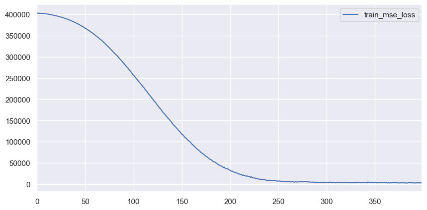
_, ax = plt.subplots(figsize=(10, 5), dpi=100)
trainer.training_info.tail(3)
trainer.training_info.plot(y=['train_mse_loss'], ax=ax)

[21]:

	total_iters	i_epoch	i_batch	train_mse_loss
397	397	398	1	3684.717041
398	398	399	1	3058.761719
399	399	400	1	3039.683350

[21]:

<matplotlib.axes._subplots.AxesSubplot at 0x1a2ce256d0>

../_images/tutorials_4-random_nn_model_and_training_37_2.png

[22]:

y_pred = trainer.predict(x_in=torch.tensor(x_val.values, dtype=torch.float)).detach().numpy().flatten()
y_true = y_val.values.flatten()

y_fit_pred = trainer.predict(x_in=torch.tensor(x_train.values, dtype=torch.float)).detach().numpy().flatten()
y_fit_true = y_train.values.flatten()

draw(y_true, y_pred, y_fit_true, y_fit_pred, prop_name='Volume ($\AA^3$)')

Missing directory and/or file name information!

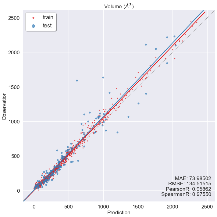
../_images/tutorials_4-random_nn_model_and_training_38_1.png

You can see that although trainer can keep training info automatically for us, we still need to convert DataFrame to torch.Tensor and convert dtype from np.double to torch.float during training, and eventually convert them back during prediction ourselves. Also, overfitting could be observed in the prediction vs observation plot. One possible caused is using all training data in each epoch of the training process. We can use a technique called mini-batch to avoid overfitting, but that will require more coding.

To skip these tedious coding steps, we provide an extension system.

First, we use ArrayDataset to wrap our data, and use torch.utils.data.DataLoader to a build mini-batch loader.

[23]:

from xenonpy.model.training.dataset import ArrayDataset
from torch.utils.data import DataLoader

[24]:

train_dataset = DataLoader(ArrayDataset(x_train, y_train), shuffle=True, batch_size=100)
val_dataset = DataLoader(ArrayDataset(x_val, y_val), batch_size=1000)

Second, we use TensorConverter extension to automatically convert data between numpy and torch.Tensor. Additionally, we want to trace some stopping criterion and use early stopping when these criterion stop improving. This can be done by using Validator.

At last, to save our model for latter use, just add Persist to the trainer and saving will be done in slient.

[25]:

from xenonpy.model.training.extension import Validator, TensorConverter, Persist
from xenonpy.model.training.dataset import ArrayDataset
from xenonpy.model.utils import regression_metrics

We use trainer.extend method to stack up extensions. Note that extensions will be executed in the order of insertion, so TensorConverter should always go first and Persist be the last.

[26]:

trainer = Trainer(
    optimizer=Adam(lr=0.01),
    loss_func=MSELoss(),
).extend(
    TensorConverter(),
    Validator(metrics_func=regression_metrics, early_stopping=30, trace_order=5, mae=0.0, pearsonr=1.0),
)

[27]:

Persist?

Init signature:
Persist(
    path: Union[pathlib.Path, str] = '.',
    *,
    model_class: Callable = None,
    model_params: Union[tuple, dict, <built-in function any>] = None,
    increment=False,
    sync_training_step=False,
    **describe: Any,
)
Docstring:      Trainer extension for data persistence
Init docstring:
Parameters
----------
path
    Path for model saving.
model_class
    A factory function for model reconstructing.
    In most case this is the model class inherits from :class:`torch.nn.Module`
model_params
    The parameters for model reconstructing.
    This can be anything but in general this is a dict which can be used as kwargs parameters.
increment
    If ``True``, dir name of path will be decorated with a auto increment number,
    e.g. use ``model_dir@1`` for ``model_dir``.
sync_training_step
    If ``True``, will save ``trainer.training_info`` at each iteration.
    Default is ``False``, only save ``trainer.training_info`` at each epoch.
describe:
    Any other information to describe this model.
    These information will be saved under model dir by name ``describe.pkl.z``.
File:           ~/projects/XenonPy/xenonpy/model/training/extension/persist.py
Type:           type
Subclasses:

Persist need a path to save model. For convenience, we prepare the path name by concatenating the number of neurons in a model.

[28]:

def make_name(model):
    name = []
    for n, m in model.named_children():
        if 'layer_' in n:
            name.append(str(m.linear.in_features))
        else:
            name.append(str(m.in_features))
            name.append(str(m.out_features))
    return '-'.join(name)

[29]:

model = SequentialLinear(290, 1, h_neurons=(0.8, 0.6, 0.4, 0.2))
model

model_name = make_name(model)
persist = Persist(
    f'trained_models/{model_name}',
    # -^- required -^-

    # -v- optional -v-
    increment=False,
    sync_training_step=True,
    author='Chang Liu',
    email='liu.chang.1865@gmail.com',
    dataset='materials project',
)
_ = trainer.extend(persist)
trainer.reset(to=model)

trainer.fit(training_dataset=train_dataset, validation_dataset=val_dataset, epochs=400)
persist(splitter=sp, data_indices=prop.index.tolist())  # <-- calling of this method only after the model training

[29]:

SequentialLinear(
  (layer_0): LinearLayer(
    (linear): Linear(in_features=290, out_features=232, bias=True)
    (dropout): Dropout(p=0.1)
    (normalizer): BatchNorm1d(232, eps=0.1, momentum=0.1, affine=True, track_running_stats=True)
    (activation): ReLU()
  )
  (layer_1): LinearLayer(
    (linear): Linear(in_features=232, out_features=174, bias=True)
    (dropout): Dropout(p=0.1)
    (normalizer): BatchNorm1d(174, eps=0.1, momentum=0.1, affine=True, track_running_stats=True)
    (activation): ReLU()
  )
  (layer_2): LinearLayer(
    (linear): Linear(in_features=174, out_features=116, bias=True)
    (dropout): Dropout(p=0.1)
    (normalizer): BatchNorm1d(116, eps=0.1, momentum=0.1, affine=True, track_running_stats=True)
    (activation): ReLU()
  )
  (layer_3): LinearLayer(
    (linear): Linear(in_features=116, out_features=58, bias=True)
    (dropout): Dropout(p=0.1)
    (normalizer): BatchNorm1d(58, eps=0.1, momentum=0.1, affine=True, track_running_stats=True)
    (activation): ReLU()
  )
  (output): Linear(in_features=58, out_features=1, bias=True)
)

Training:  12%|█▏        | 47/400 [00:15<02:06,  2.78it/s]

Early stopping is applied: no improvement for ['mae', 'pearsonr'] since the last 31 iterations, finish training at iteration 372

[30]:

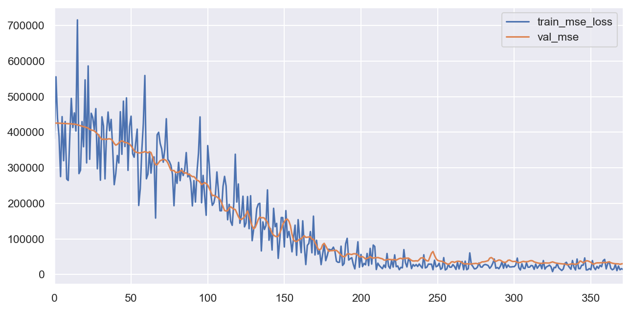
_, ax = plt.subplots(figsize=(10, 5), dpi=150)
trainer.training_info.plot(y=['train_mse_loss', 'val_mse'], ax=ax)

[30]:

<matplotlib.axes._subplots.AxesSubplot at 0x1a2d100e10>

../_images/tutorials_4-random_nn_model_and_training_51_1.png

[31]:

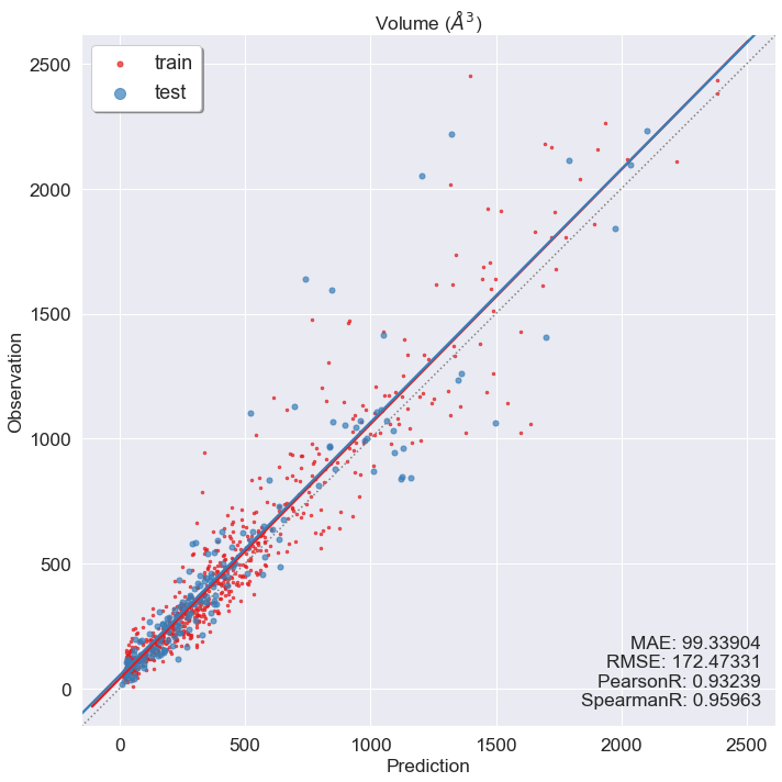
y_pred, y_true = trainer.predict(dataset=val_dataset, checkpoint='pearsonr_1')
y_fit_pred, y_fit_true = trainer.predict(dataset=train_dataset, checkpoint='pearsonr_1')
draw(y_true, y_pred, y_fit_true, y_fit_pred, prop_name='Volume ($\AA^3$)')

Missing directory and/or file name information!

../_images/tutorials_4-random_nn_model_and_training_52_1.png

Combine random model generating and training

[32]:

generator = ParameterGenerator(
    in_features=290,
    out_features=1,
    h_neurons=dict(
        data=lambda n: sorted(np.random.uniform(0.2, 0.8, size=n), reverse=True),
        repeat=(3, 4)
    )
)

[33]:

for paras, model in generator(num=2, factory=SequentialLinear):
    print(model)
    model_name = make_name(model)
    persist = Persist(
        f'trained_models/{model_name}',
        # -^- required -^-

        # -v- optional -v-
        increment=False,
        sync_training_step=True,
        model_class=SequentialLinear,
        model_params=paras,
        author='Chang Liu',
        email='liu.chang.1865@gmail.com',
        dataset='materials project',
    )
    _ = trainer.extend(persist)
    trainer.reset(to=model)

    trainer.fit(training_dataset=train_dataset, validation_dataset=val_dataset, epochs=400)
    persist(splitter=sp, data_indices=prop.index.tolist())  # <-- calling of this method only after the model training

Training:   0%|          | 0/400 [00:00<?, ?it/s]

SequentialLinear(
  (layer_0): LinearLayer(
    (linear): Linear(in_features=290, out_features=195, bias=True)
    (dropout): Dropout(p=0.1)
    (normalizer): BatchNorm1d(195, eps=0.1, momentum=0.1, affine=True, track_running_stats=True)
    (activation): ReLU()
  )
  (layer_1): LinearLayer(
    (linear): Linear(in_features=195, out_features=141, bias=True)
    (dropout): Dropout(p=0.1)
    (normalizer): BatchNorm1d(141, eps=0.1, momentum=0.1, affine=True, track_running_stats=True)
    (activation): ReLU()
  )
  (layer_2): LinearLayer(
    (linear): Linear(in_features=141, out_features=131, bias=True)
    (dropout): Dropout(p=0.1)
    (normalizer): BatchNorm1d(131, eps=0.1, momentum=0.1, affine=True, track_running_stats=True)
    (activation): ReLU()
  )
  (layer_3): LinearLayer(
    (linear): Linear(in_features=131, out_features=61, bias=True)
    (dropout): Dropout(p=0.1)
    (normalizer): BatchNorm1d(61, eps=0.1, momentum=0.1, affine=True, track_running_stats=True)
    (activation): ReLU()
  )
  (output): Linear(in_features=61, out_features=1, bias=True)
)

Training:  12%|█▏        | 48/400 [00:15<02:06,  2.79it/s]
Training:   0%|          | 0/400 [00:00<?, ?it/s]

Early stopping is applied: no improvement for ['mae', 'pearsonr'] since the last 31 iterations, finish training at iteration 380
SequentialLinear(
  (layer_0): LinearLayer(
    (linear): Linear(in_features=290, out_features=214, bias=True)
    (dropout): Dropout(p=0.1)
    (normalizer): BatchNorm1d(214, eps=0.1, momentum=0.1, affine=True, track_running_stats=True)
    (activation): ReLU()
  )
  (layer_1): LinearLayer(
    (linear): Linear(in_features=214, out_features=181, bias=True)
    (dropout): Dropout(p=0.1)
    (normalizer): BatchNorm1d(181, eps=0.1, momentum=0.1, affine=True, track_running_stats=True)
    (activation): ReLU()
  )
  (layer_2): LinearLayer(
    (linear): Linear(in_features=181, out_features=141, bias=True)
    (dropout): Dropout(p=0.1)
    (normalizer): BatchNorm1d(141, eps=0.1, momentum=0.1, affine=True, track_running_stats=True)
    (activation): ReLU()
  )
  (layer_3): LinearLayer(
    (linear): Linear(in_features=141, out_features=130, bias=True)
    (dropout): Dropout(p=0.1)
    (normalizer): BatchNorm1d(130, eps=0.1, momentum=0.1, affine=True, track_running_stats=True)
    (activation): ReLU()
  )
  (output): Linear(in_features=130, out_features=1, bias=True)
)

Training:  10%|█         | 42/400 [00:14<02:18,  2.59it/s]

Early stopping is applied: no improvement for ['mae', 'pearsonr'] since the last 31 iterations, finish training at iteration 333

[ ]: